Algorithm Analysis and Big O Notation

When we're programming, we're writing code to perform a specific task. An algorithm is a set of instructions - the procedure we ask the computer to perform - to complete that task.

For any task, there are a huge number of possible algorithms we can write to complete it. How do we decide on which one to use?

Typically, one of the main considerations we have is that we generally prefer algorithms that require fewer actions to complete. An algorithm that requires fewer instructions to complete its task is generally going to be able to complete that task faster.

Being conscious of the performance of our algorithms is particularly important in two scenarios:

1. Real-Time Graphics

If we are writing a program that involves real-time interactivity, we typically want to update the user's screen at least 60 times per second to make our application feel responsive.

This gives us approximately 16 milliseconds to generate each update. If one of the algorithms we use in that process takes 10 milliseconds, most of our budget is immediately gone.

2. Big Data

In other contexts, we might not be dealing with short timeframes - rather, we might be dealing with large amounts of data. If we're creating software that analyses a billion records, and our algorithm spends 10 milliseconds on each record, our program will take four months to run.

Algorithm Scaling

Generally, how long our algorithms take to run will depend on their inputs, specifically, the size of those inputs.

Our input's size might be the number of pixels we need to color, or the number of records we need to process. When the input is larger, our algorithms typically need to do more work.

The main thing we care about is how the input size affects the number of operations our algorithm needs to perform. As our input size increases, how many more operations does our algorithm need to perform to complete its task?

This is referred to as the scaling of our algorithm. Below, we provide examples of the most common scaling factors:

Constant Scaling

This is the best-case scenario. With constant scaling, even if our input gets bigger, our algorithm doesn't need to do any extra work. An example of a problem that can be solved in constant time is: "determine if the first element in an array of numbers is even"

1bool FirstIsEven(std::vector<int>& Input) {
2  return Input[0] % 2 == 0;
3}

Here, it doesn't matter how big the input array is - our algorithm takes the same, constant, amount of time.

Linear Scaling

With linear scaling, as our input gets bigger, our algorithm needs to perform proportionally more work. If our input is twice as large, our algorithm needs to do approximately twice as much work.

An example of a problem that can be solved in linear time is: determine how many numbers in an array are even. To solve this, we need to inspect every element in the array.

If the array is twice as large, we need to do approximately twice as much work. We can often identify a linear algorithm by the fact it iterates over every object in our collection:

1int CountEven(const std::vector<int>& Input) {
2  int Total { 0 };
3  for (int i : Input) {
4    if (i % 2 == 0) ++Total;
5  }
6  return Total;
7}

Here, if the array has 10 items, the highlighted line is executed 10 times. If the array is doubled to 20 items, the number of times the line is executed is also doubled to 20. In other words, the number of operations scales linearly with the size of the input.

Quadratic Scaling and Beyond

Algorithms in this category tend to involve nested loops. Let's imagine we have the task: "check if an array contains any duplicates"

We'll introduce a better way to solve this problem in the next lesson, but one possible solution we might consider would be to use nested loops:

1bool HasDuplicate(std::vector<int>& Input) {
2  for (size_t i{0}; i < Input.size(); ++i) {
3    for (size_t j{0}; j < Input.size(); ++j) {
4      if (Input[i] == Input[j] && i != j) {
5        return true;
6      }
7    }
8  }
9  return false;
10}

In this example, if our input array has 10 items, the outer for loop performs 10 iterations, and each iteration causes the inner for loop to perform 10 iterations.

The net effect is that the highlighted if statement is evaluated up to 100 times - 10 x 10.

If the array is increased to 100 items, the if block is now executed up to 10,000 times. With quadratic scaling, the number of operations increases much faster than the size of the input.

In general, if our input contains $n$ objects, this algorithm requires $n \times n$, or $n^2$ operations to complete its task. This is an example of quadratic scaling.

We could also have cubic algorithms that require $n \times n \times n$, or $n^3$ operations. This would be the case had we needed a 3rd nested loop:

1for (int i : Input) {
2  for (int j : Input) {
3    for (int k : Input) {
4      // Code here will run n * n * n times
5    }
6  }
7}

This pattern continues - there are quartic algorithms requiring $n^4$ operations, and so on.

Algorithm Scaling Compared

The following chart is a visual representation of how many operations an algorithm in each of these classifications might need to perform.

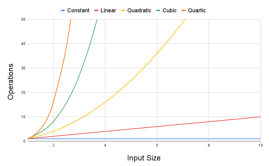
If we zoom out in this chart, we can see the differences can get quite extreme:

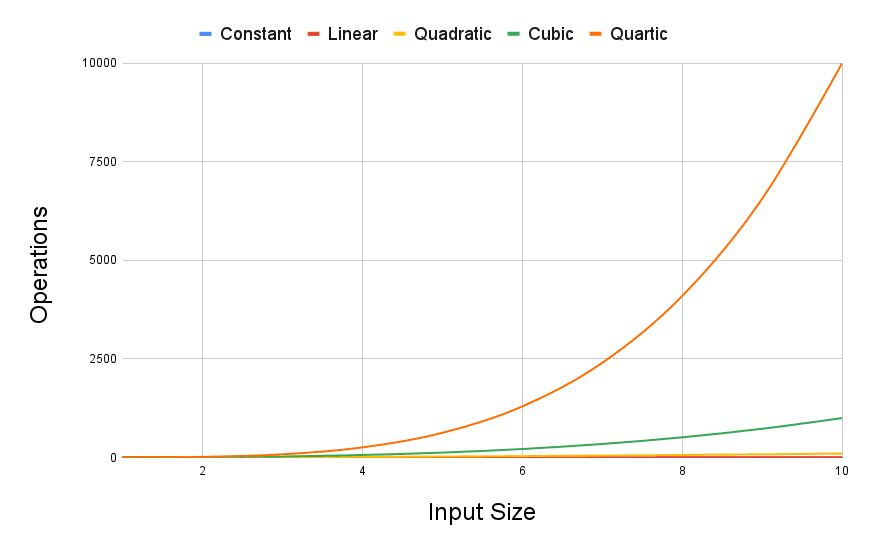
Even with a modest input size of 10, the huge differences in each type of algorithm are clear.

Big O Notation

The concept of "Big O" is a mathematical notation that is used to represent the concepts covered above.

We can imagine the algorithms we create as being within certain classes of scaling:

• Constant algorithms are noted as $O(1)$
• Linear algorithms are noted as $O(n)$
• Quadratic algorithms are noted as $O(n^2)$, and so on.

It is quite rare that the algorithms we create to solve real-world problems fit exactly into these equations. For example, an algorithm might have $50n^2$ operations. Another might require $n^2 + 10n + 30$ operations.

Big O notation simplifies things to just the core classification - both of these algorithms would be $O(n^2)$. This simplification allows us to communicate and compare approaches more simply.

Specifically, it makes the following simplifications:

1. Treat all operations as equal

In the real world, some operations can take much more time than others. For example, CPUs can perform multiplication faster than division and can read data from memory faster than from the hard drive.

But to keep things simple, we assume all operations are equally fast

2. Ignore Constants

One algorithm might require $n + 100$ operations whilst another might require $n$. We ignore the additive constant - both these algorithms are in the same class - $O(n)$ (linear)

One algorithm might require $50n$ operations whilst another might require $n$. We also ignore multiplicative constants - these algorithms are still both in the same class - $O(n)$ (linear)

3. Only Include the Dominant Term

One algorithm might require $n^2 + n$ operations whilst another might require $n^2 + 50$. As we saw in the graphs above, the term with the highest order (that is, the largest exponent) dominates the behavior of the function as $n$ increases

Because of this, we just ignore all the lower-order terms. Both of these algorithms are simply $O(n^2)$ (quadratic)

Operations vs Statements

It's important not to confuse the number of operations an algorithm performs with the number of statements it has.

The following function contains a single statement, but that doesn't necessarily mean the function has a constant run time. To understand the time complexity of HandleArray(), we would need to understand the time complexity of the function it calls:

1void HandleArray(std::vector<int>& Input) {
2  SomeFunction(Input); // ? 
3}

If SomeFunction() is linear, requiring $n$ operations, then HandleArray() would also be linear.

In the following example, if SomeFunction() is linear, then HandleArray() will be quadratic, requiring $n \times n$, or $n^2$ operations:

1void HandleArray(std::vector<int>& Input) {
2  for (int x : Input) {
3    SomeFuncion(Input, x);
4  }
5}

Remember, operators are also functions. So, to understand the time complexity of this function, we need to understand the time complexity of SomeType::operator+=(int):

1void Add(SomeType& Input) {
2  Input += 1; // ? 
3}

When we're using third-party functions, the time complexity will often be listed in the documentation.

The complexity of standard library functions will be listed in most online references. For example, cppreference.com lists the complexity of std::vector's erase() method as linear.

Summary

In this lesson, we explored the fundamentals of algorithm analysis and Big O notation, understanding how different algorithms scale with input size and how to categorize their efficiency in terms of time complexity.

Key Takeaways:

• Algorithms vary in efficiency; their performance is often measured using time complexity, with Big O notation providing a standardized way to express this.
• We examined constant, linear, and quadratic scaling, highlighting how the size of input impacts the number of operations in an algorithm.
• Big O notation simplifies algorithm complexity by focusing on the dominant term and ignoring constants and lower-order terms.
• The distinction between operations and statements in code was clarified, emphasizing the need to understand the complexity of underlying functions.

Next Lesson Preview: Data Structures

In our upcoming lesson, we'll dive into the world of data structures. We'll explore how different data structures can significantly impact the performance and efficiency of algorithms, building upon the concepts of algorithm analysis and Big O notation discussed in this lesson.

Key Topics:

• Introduction to Common Data Structures: Learn how arrays compare to two other common data structures - the hash set and the linked list.
• Impact on Algorithm Efficiency: Understand how the choice of a data structure can affect an algorithm's time complexity and overall performance.
• Improving Algorithms using Data Structures: We'll learn how data structures can work together to create more efficient algorithms.
• Practical Examples: We'll add a new data structure to the HasDuplicate() function from this lesson, to improve its run time from $O(n^2)$ to $O(n)$

Free and Unlimited Access

Professional C++

Unlock the true power of C++ by mastering complex features, optimizing performance, and learning expert workflows used in professional development

View Course