In previous lessons, we handled transformations between spaces by writing custom C++ functions. We manually multiplied coordinates by scale factors and added offsets to move them around.

While this works for simple cases, when working in more complex projects, it is tremendously helpful to have a unified framework to describe and apply transformations to sets of points in our world, or the entire world itself.

Transformation Matrices

In higher-budget games and engines, transformations are implemented using matrices and matrix multiplication. These are core concepts from Linear Algebra, the branch of mathematics concerning vectors, vector spaces, and linear mappings.

We'll focus more on the practical application in the next two lessons. If you are interested in a deep dive into the mathematics behind this, 3Blue1Brown has a visual series on the topic on YouTube

The objectives remain the same as our previous custom functions: we want a unified way to move, rotate, and scale objects. The difference is the mechanism.

Rather than writing a function like ToScreenSpace(x, y), we define a Matrix - a grid of numbers that represents the transformation mathematically.

For example, our previous manual calculation:

1// Define the transformation
2Vec2 ToScreenSpace(const Vec2& Pos) {
3  return {
4    Pos.x * 0.5f,           // Scale X
5    (Pos.y * -0.5f) + 300   // Scale Y and Translate Y
6  };
7}

Can be represented by this matrix:

\begin{bmatrix} 0.5 & 0 & 0 \\ 0 & -0.5 & 300 \\ 0 & 0 & 1 \end{bmatrix}

You can see the numbers from our function (0.5, -0.5, and 300) included in this matrix, and their position within the matrix represents how those numbers are used.

We don't need to understand exactly how to position our values as, in practice, we don't create these matrices by hand. We enlist the help of a library which lets us define our matrix through functions with helpful names like scale(), translate(), and rotate().

Creating this matrix using GLM, which we'll introduce in the next lesson, looks like this:

1#include <glm/glm.hpp>
2#include <glm/gtc/matrix_transform.hpp>
3
4// create an "empty" transformation matrix
5glm::mat3 m(1.0f);
6
7// update it to include a (0.5, -0.5) scaling
8m = glm::scale(transform, glm::vec2(0.5f, -0.5f));
9
10// update it to include a (0, 300) translation
11m = glm::translate(transform, glm::vec2(0.0f, 300.0f));

Homogeneous Coordinates

You might notice something odd here. We are working with 2D coordinates ( $x$ and $y$ ), but our matrix is $3 \times 3$ . This brings us to an important concept.

To support the full range of transformations we typically need using matrix multiplication, we cannot simply use a $2 \times 2$ matrix for 2D space.

To solve this, we increase the dimension of our data by one.

In a 2D game, we use 3D vectors, and 3x3 transformation matrices.
In a 3D game, we use 4D vectors and 4x4 transformation matricies.

This system is called homogeneous coordinates.

The `w` Component

When we upgrade our vector, our additional coordinate is generally called $w$ (or sometimes $h$ ). In 2D:

\begin{bmatrix} x \\ y \end{bmatrix} \rightarrow \begin{bmatrix} x \\ y \\ w \end{bmatrix}

In 3D:

\begin{bmatrix} x \\ y \\ z \end{bmatrix} \rightarrow \begin{bmatrix} x \\ y \\ z \\ w \end{bmatrix}

The value of $w$ determines how much the vector is affected by translations coming from a transformation matrix. In practice, the value of $w$ is usually either 1 or 0.

If we set it to 1, we signal that we want the vector to be fully affected by translations. This typically means the vector is being used to represent a position.

If we use 0, translations are effectively ignored by that vector. That is typically what we want for vectors that represent relative or directional concepts. Typical examples include what direction an object is facing, its velocity, or its acceleration.

Practical Example: The Player Character

Imagine a player character in a game world. This character has three distinct vectors defining their state. Note that we don't have this hypothetical Vec3 type yet, but the GLM library we use in the next lesson provides something similar:

1class Player {
2public:
3  // The player starts at (100, 50)
4  // This is a position, so we add w = 1
5  Vec3 Position{100, 50, 1};
6  
7  // Moving right at 10 units per tick
8  // Velocity is not a position - it is a relative
9  // concept, so we add w = 0
10  Vec3 Velocity{10, 0, 0};
11  
12  // The player is looking "up" (positive Y)
13  // This is also not a position - it is a direction
14  // so we add w = 0
15  Vec3 Facing{0, 1, 0};
16}

Now, imagine we apply a transformation that moves everything in the world by $+500$ in the $x$ direction.

The character's Position had $w = 1$ , so we want the character to by physically moved by this transformation. It's position should be updated to $(600, 50)$ .
The Velocity had $w = 0$ , so we want the translation to be ignored for this vector. Just because the character is in a different part of the map, they shouldn't suddenly be moving faster.
The Facing also had $w = 0$ , so the translation should be ignored. They should still be looking up.

Note that setting $w = 0$ means that the vector only ignores translations. It still respects other transformations, such as rotations and reflections.

If the transformation flipped our world such that the $y$ axis pointed "down", then Facing would be transformed from $(0, 1, 0)$ to $(0, -1, 0)$ .

The Player would still be facing "up" after that transformation - it's just that we're now in a space where the definition of "up" has changed from positive Y to negative Y

Advanced: Linear and Affine Transformations

Mathematically, a simple matrix multiplication (without the extra dimension) represents a linear transformation. Linear transformations have a restrictive property: they cannot move the origin. They can stretch, squash, and rotate space, but they cannot move (translate) the space.

Translations are affine transformations. Affine transformations combines can combine all the possible linear transformation, but they can also include translation.

By moving to homogeneous coordinates (adding the $w$ dimension), we can represent affine transformations in 2D space as linear transformations in 3D space, or affine transformations in 3D space as linear transformations in 4D space.

For our 2D example, we can imagine our 2D space being a plane at $w=1$ in a 3D space. This is often visualized as our 2D world existing on the top surface of a cube:

Diagram showing the 2D plane represented within 3D space

A "shear" operation in 3D space is a linear transformation that doesn't move the origin. However, it looks exactly like a translation when we consider only how it affects the 2D space we care about - the plane at $w = 1$ .

Diagram showing the affine transformation

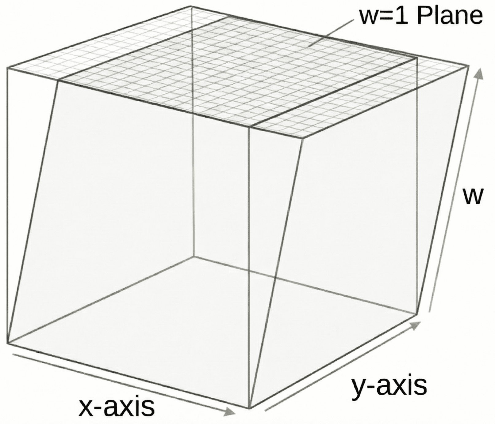
This diagram also helps illustrate why setting $w = 0$ represents a desire to ignore translation. A vector with a $w$ value of $0$ is at the base of this cube, which is not moved by this transformation.

This mathematical trick unifies all movement and transformation into a single system: matrix multiplication. This unification is powerful because it means a single math operation (and a single piece of hardware on the GPU) can handle any combination of movement, rotation, and sizing.

The idea of a lower dimension space being a "projection" within a higher dimension space allows us to create even more exotic transformations than these. The most notable example is the perspective projection transformation we introduced in the previous lesson, which creates the illusion that distant objects appear smaller.

Matrix Multiplication

When our transformation was defined as a function, applying it was obvious - we simply call the function, passing the vector we want to be transformed.

To modify a vector using a transformation represented as a matrix, we perform matrix multiplication: we multiply our transformation matrix by our vector. A vector is also a matrix - it has only one row or, more commonly, it is arranged vertically to create a matrix with only one column. For example, $(700, 300, 1)$ can be represented as the following column vector:

\begin{bmatrix} 700 \\ 300 \\ 1 \end{bmatrix}

We don't need to fully understand matrix multiplication to implement it. Again, we'll enlist a library to help with this. But, if you do need to perform a matrix multiplication outside of code, or to visualize how the algorithm works, http://matrixmultiplication.xyz/ demonstrates exactly how the rows and columns of our matrices combine to produce the result of the multiplication. Note that, for the multiplication to work correctly, our vector must be presented as a column rather than a row.

In our context, if we want to transform a position of $(700, 300)$ , we set up the column vector with $w=1$ and multiply:

\begin{bmatrix} 0.5 & 0 & 0 \\ 0 & -0.5 & 300 \\ 0 & 0 & 1 \end{bmatrix} \cdot \begin{bmatrix} 700 \\ 300 \\ 1 \end{bmatrix} = \begin{bmatrix} 350 \\ 150 \\ 1 \end{bmatrix}

The result is a new vector $x=350, y=150$ which matches the output of our helper function from the previous lesson perfectly.

Why use Matrices?

Comparing this to our earlier simple function, the matrix approach has massive advantages:

Composability: Transformation matrices can also be multiplied by other transformation matrices. This creates a new, single matrix that combines both transformations. We can combine as many transformations as we need (rotation, scaling, shearing, translation) in this way. We can then apply our final "master matrix" to a million points to transform each of them in a single step.
Hardware Acceleration: When we unify our transformation process using this standardised technique, we can then take advantage of hardware acceleration. GPUs are designed specifically to perform matrix multiplication. Passing a matrix to the graphics card is significantly faster than calculating positions on the CPU.
Standardization: Using standard matrix logic makes our code compatible with many other systems, such as physics engines, graphics APIs, and other tools

In the next lesson, we will move to implementing this system in our C++ code with help from the GLM library.

Matrix Transformations and Homogeneous Coordinates

Transformation Matrices

Homogeneous Coordinates

The `w` Component

Practical Example: The Player Character

Advanced: Linear and Affine Transformations

Matrix Multiplication

Why use Matrices?

The GLM Library

Game Development with SDL3

Matrix Transformations and Homogeneous Coordinates

Transformation Matrices

Homogeneous Coordinates

The w Component

Practical Example: The Player Character

Advanced: Linear and Affine Transformations

Matrix Multiplication

Why use Matrices?

The GLM Library

The `w` Component